Summarize GPS information in a regular grid

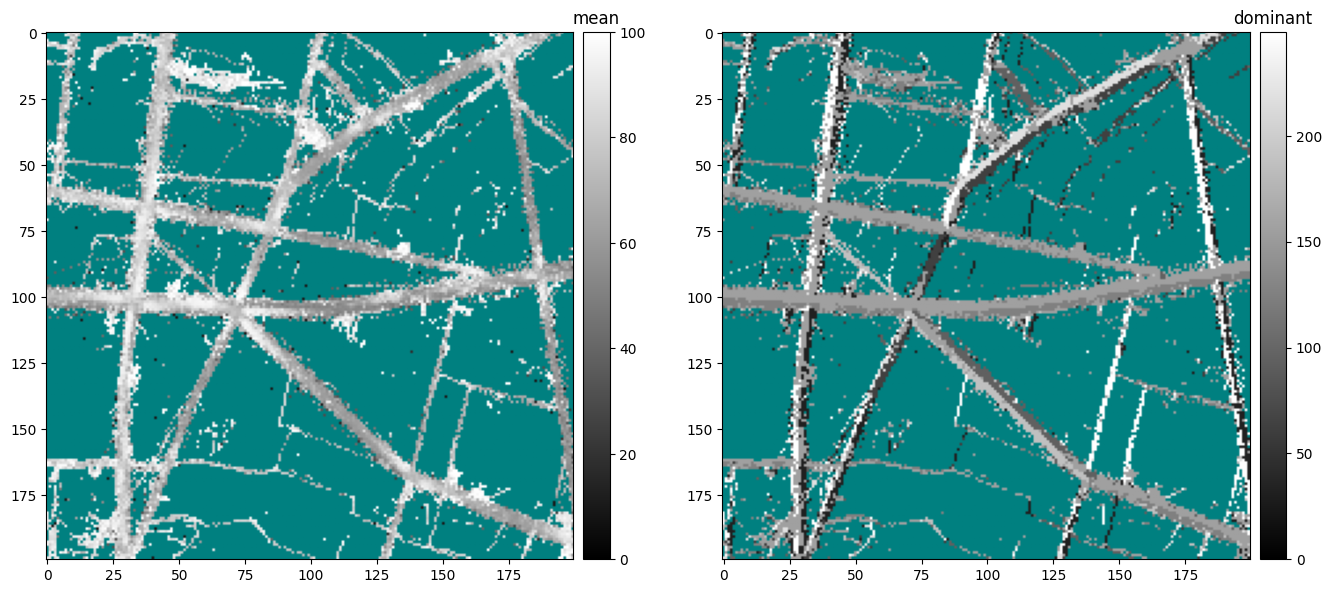
This functionality of tracklib reduce the full dataset of GPS traces into a regular grid of summarized features. In each cell, n aggregated features (such as mean and standard deviation of speeds, number of traces, most frequent bearing …) are computed to produce a set of raster maps, which may be seen as a single image with n channels.

These process has been used in works presented in (1).

Figure 1 : Workflow presented in (1) to produce raster images (5 meter-resolution grid)

Reference:(1) - Y. Méneroux and al. Convolutional Neural Network for Traffic Signal Inference based on GPS Traces. Proceedings of Spatial big data and machine learning in GIScience Workshop’18, August 28-31, 2018, Melbourne, Australia. GIScience.

Importing Tracklib

# -*- coding: utf-8 -*-
import os.path
import sys

# Import the Tracklib library
import tracklib as trk

# Import plotting library
import matplotlib.pyplot as plt

Code running in a no shapely environment

Chargement du jeu de traces

The dataset comprises a set of 11862 GPS traces, located in Mitaka city (16 km2), suburbs of Tokyo (Japan).

PATH = '../../../../../PROJET/FINI/MITAKA/DATA/mitaka/complet'
trk.ObsTime.setReadFormat("4Y-2M-2D 2h:2m:2s")
param = trk.TrackFormat({
    'ext': 'CSV',
    'id_E':2,
    'id_N':3,
    'id_T':1
})
collection = trk.TrackReader.readFromFile(PATH, param)
print ('Number of tracks: ' + str(collection.size()))

Number of tracks: 11872

Sélection des traces sur une zone restreinte de type Rectangle

import matplotlib.pyplot as plt

Xmin = 370250
Xmax = 371250
Ymin = 3949050
Ymax = 3950050

ll = trk.ENUCoords(Xmin, Ymin)
ur = trk.ENUCoords(Xmax, Ymax)
bbox = trk.Rectangle(ll, ur)

constraintBBox = trk.Constraint(shape = bbox, mode = trk.MODE_INSIDE, type=trk.TYPE_CUT_AND_SELECT)
selections = constraintBBox.select(collection)
print ('Number of tracks: ' + str(selections.size()))

for track in selections:
    if track.size() < 10:
        selections.removeTrack(track)
selections.plot('k')

plt.xlim((Xmin, Xmax))
plt.ylim((Ymin, Ymax))
plt.show()

print ('Number of tracks: ' + str(selections.size()))
collection = selections

Number of tracks: 3850

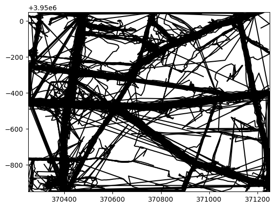
Number of tracks: 3802

Raster de la moyenne des vitesses et de l’orientation de la plus fréquente par cellule

Les AF seront calculées si elles n’ont pas encore été créées

Les scripts des deux AF qu’on prend existent déjà dans la librairie, sinon il aurait fallu les écrire

# On crée l'AF speed
collection.addAnalyticalFeature(trk.speed)
collection.addAnalyticalFeature(trk.orientation)

# On crée le raster (emprise, résolution)
margin = 0
resolution = (5, 5)
raster = trk.Raster(bbox=collection.bbox(), resolution=resolution, margin=margin,
                        align=trk.BBOX_ALIGN_CENTER)

# On ajoute les AF avec les agrégats
speedMap = raster.addAFMap("speed")
speedMap.addMean()

bearingMap = raster.addAFMap("orientation")
bearingMap.addDominant()

# On lance l'affectation des observations dans la grille, puis les calculs
trk.summarize(collection, raster)

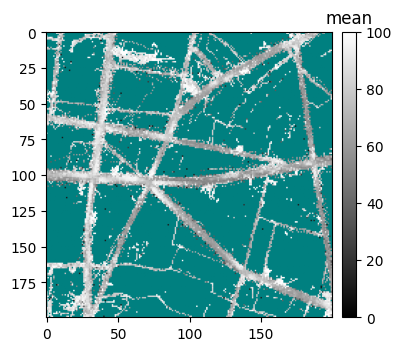
Conversion des indicateurs en 8-bit grayscale

Feature values are converted on a 8-bit grayscale.

# the mean of speeds is distributed between 16 and 255
for i in range(raster.nrow):
    for j in range(raster.ncol):
        val = speedMap['mean'].getGrid().values[i][j]
        if val != raster.getNoDataValue():
            if val > 25:
                speedMap['mean'].getGrid().values[i][j] = 10
            else:
                speedMap['mean'].getGrid().values[i][j] = 100 - val/25*90


# The dominance of orientations is discretized in 8 eight values
for i in range(raster.nrow):
    for j in range(raster.ncol):
        val = bearingMap['dominant'].getGrid().values[i][j]
        if val != raster.getNoDataValue():
            if val == 1:
                bearingMap['dominant'].getGrid().values[i][j] = 156
            elif val == 2:
                bearingMap['dominant'].getGrid().values[i][j] = 218
            elif val == 3:
                bearingMap['dominant'].getGrid().values[i][j] = 249
            elif val == 4:
                bearingMap['dominant'].getGrid().values[i][j] = 187
            elif val == 5:
                bearingMap['dominant'].getGrid().values[i][j] = 125
            elif val == 6:
                bearingMap['dominant'].getGrid().values[i][j] = 63
            elif val == 7:
                bearingMap['dominant'].getGrid().values[i][j] = 32
            elif val == 8:
                bearingMap['dominant'].getGrid().values[i][j] = 94
            else:
                bearingMap['dominant'].getGrid().values[i][j] = 0

Affichage

import matplotlib.pyplot as plt

# make an image, just to create the icon for the use case gallery
color1 = (0, 0, 0)
color2 = (255, 255, 255)
cmap = trk.getOffsetColorMap(color1, color2, 0)
cmap.set_bad(color='teal')

fig, ax1 = plt.subplots(figsize=(4, 4))

speedMap.plot(band='mean', cmap=cmap, vmin=0, append=ax1)
plt.show()

fig = plt.figure(figsize=(16, 8))

ax1 = fig.add_subplot(121)
speedMap.plot(band='mean', cmap=cmap, vmin=0, append=ax1)

ax2 = fig.add_subplot(122)
bearingMap.plot(band='dominant', cmap=cmap, vmin=0, append=ax2)
print ('')